

When an OEM receives a shipment of cells from a supplier, it must decide whether to accept or reject the lot based on inspecting a sample. This process is known as acceptance sampling.
Acceptance sampling was formalized about a century ago at Bell Laboratories, motivated by the need to inspect incoming manufactured components without testing every unit. The field was widely adopted during World War II, when the U.S. military used standardized sampling tables to qualify ammunition and equipment. After the war, these tables were codified as MIL-STD-105.
Acceptance sampling primarily addresses three points:
- How many units to inspect (n)
- How many defects to allow before rejecting the lot (c)
- What level of statistical confidence the resulting decision carries
Here, we introduce the standard acceptance sampling frameworks and explain how to choose a sample size for lot acceptance.
Acceptance Sampling Standards: AQL and LTPD
The most widely used acceptance sampling standards are ISO 2859-1 (international version) and ANSI/ASQ Z1.4 (equivalent American version). Both are indexed by the Acceptance Quality Limit (AQL, formerly “acceptable quality level”): the worst process average considered acceptable over a continuing series of lots. For a given lot size and AQL, these standards specify a sampling plan (how many units to inspect and how many defects to allow), along with rules for switching between normal, tightened, and reduced inspection as supplier history accumulates.
Every sampling plan balances two risks. Producer’s risk is the chance of rejecting a good lot, while consumer’s risk (β) is the chance of accepting a bad lot. These risks are naturally in tension: for a fixed sample size, tightening the acceptance criteria lowers consumer’s risk but raises producer’s risk, and loosening them does the opposite. The only way to reduce both at once is to inspect more cells (or extract more information from each one). Consumer’s risk is the probability of accepting a lot at a specified poor quality level, often defined using Lot Tolerance Percent Defective (LTPD). Here, for incoming inspection of safety-critical cells, we focus on consumer’s risk, or limiting the probability of accepting a lot whose defect rate is at or above the selected threshold.
A lot is defined as a distinct population of parts from a common production provenance. Typically, a lot is a single supplier shipment, production run, or a batch as defined by some other process control grouping. Lot acceptance sampling assumes the lot is a homogeneous population; mixing cells from different populations (e.g., different production lines) can dilute a problem in one population below the detection threshold. For instance, a 5% defect rate on one line would appear to be 1% when mixed with four equally sized clean lines. Precisely defining a lot can be challenging at times, but we suggest erring toward defining a lot with high granularity to maximize the chances of defect detection, at the cost of more total inspections, since the required sample size decreases only slightly with lot size (as we’ll discuss shortly).
For safety-critical defects, a zero-tolerance policy is appropriate: the lot should be rejected if even one defective cell is found in the sample. This is known as a zero-acceptance-number (c = 0) plan. A c = 0 plan rejects the lot on the first defect found. It is not the only option: for warranty-relevant defects where a small nonzero failure rate is acceptable, plans indexed to higher AQL values (often 1.5% or 4%) allow larger acceptance numbers (c > 0). For safety-critical battery failures, however, we strongly recommend the zero-tolerance c = 0 plan. Note that passing a c = 0 plan does not mean the lot is defect-free; it means the lot’s defect rate is unlikely to exceed a chosen threshold, as described below.
What About 100% Inspection?
Both battery producers and OEMs often perform 100% inspection for inexpensive techniques such as open-circuit voltage (OCV) measurements. 100% inspection for advanced techniques such as CT may make sense in some cases, particularly for small lots in applications where a single cell failure is extremely costly. For instance, satellite producers might choose 100% inspection given both their relatively small cell volumes and the enormous cost of cell failure for this application. Glimpse is working hard to speed up cell CT to seconds per cell, which will unlock 100% inspection via CT for more use cases.
However, inspecting every cell via CT is often prohibitively expensive at scale. A full CT scan of a 100,000-cell lot would take months of continuous scanning, even at the 2 minutes per cell that Glimpse achieves on conventional CT scanners. Even world-class manufacturers sample rather than rely on 100% inspection for these techniques. Tesla, for example, states that “X-ray scans are performed on 100% of cells, and CT scanning is performed on a significant fraction of cells to catch internal defects that are invisible from the outside.”
The intuition behind sampling is the same as polling. A well-designed poll of roughly 1,000 voters can estimate the preferences of 330 million Americans to within a few percentage points. The same principle applies here: inspecting a carefully chosen random sample of cells characterizes the full lot with quantifiable confidence. The key requirements are that the sample is drawn randomly and the desired confidence level is specified in advance. One key difference: a poll estimates a proportion, whereas lot acceptance tests whether the defect rate is below a threshold, which requires a different calculation (see Detection Probability).
Overall, for most applications, we recommend sampling instead of 100% inspection when using relatively expensive but information-rich techniques such as CT scanning.
Out of Scope: Pass/Fail Criteria
We do not address here how to define what constitutes a defective cell. That determination involves two separate decisions:
- The choice of test method(s). Options include OCV, AC internal resistance, capacity, visual inspection, CT scanning, and others.
- The specification thresholds that separate passing and failing cells, such as, for instance, the minimum anode overhang spec.
Both require application-specific engineering judgment and are out of scope here, although Glimpse often suggests reasonable thresholds for a given customer application. Here, we only address the statistical question of how many cells to sample given clear pass/fail criteria.
We also assume the test method catches every defective cell it inspects; in practice, the method’s detection sensitivity reduces the effective detection probability, whether you sample or inspect 100% of cells.
Confidence as a Function of Sample Size and Lot Size
The chart below answers the following question: given n cells inspected with zero defects found, what is the 95% upper bound on the true defect rate? Confidence in the lot acceptance decision increases with sample size. All curves assume zero defects were found; finding any defect immediately triggers lot rejection under the c = 0 plan.
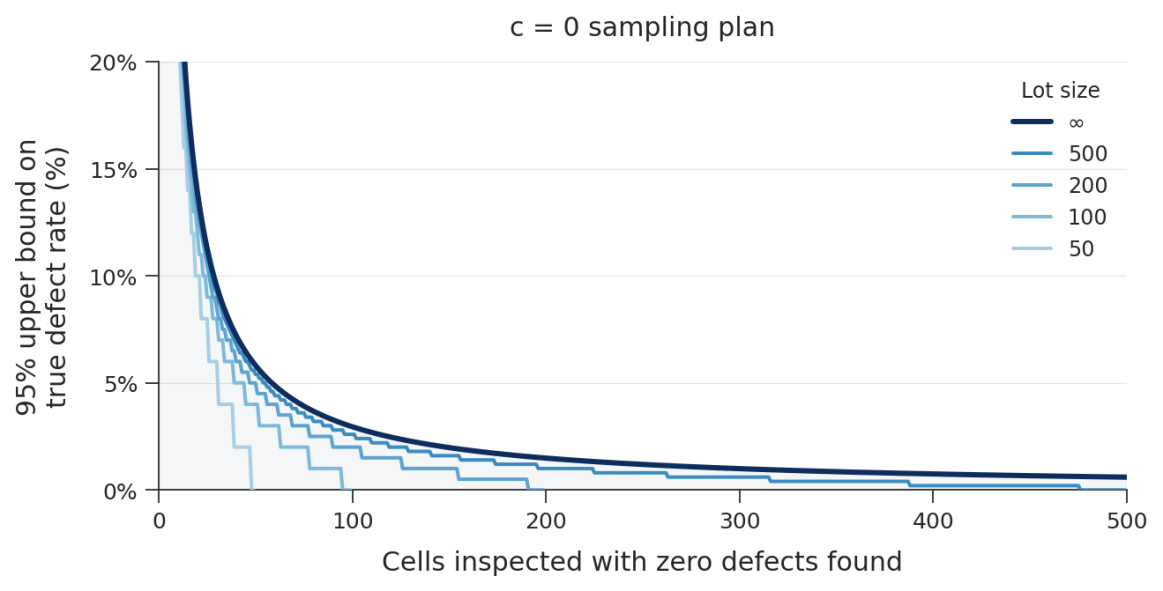
At infinite lot size, we use the binomial distribution to define this relationship. The binomial distribution is the same relationship used to model a series of independent coin flips. For finite lots, a more advanced model known as the hypergeometric model gives the exact answer. The hypergeometric model gives a tighter (more favorable) bound than the binomial, because each inspected cell directly reduces the uninspected remainder. As expected, fewer samples are required to bound a defect rate for a lot with 50 cells as opposed to 100,000 cells. That said, for practical lot sizes of N ≥ 1,000 and n ≤ 100, the binomial is an excellent approximation.
The 95% confidence level is a convention, not a requirement. Using 90% confidence reduces the required sample size by about 23%; using 99% increases it by about 54%. The same framework applies at any confidence level by replacing 0.05 with the chosen consumer’s risk β (β = 1 − confidence level) in the formula pupper = 1 − β1/n (see the Appendix).
Sample Size Reference Tables
The tables below show the minimum number of cells to inspect (with zero defects found) to bound the true defect rate below each threshold at both 95% and 99% confidence. For finite lots, the sample size is chosen so that any lot with a defect rate at or above the threshold is rejected with at least the stated confidence. For example, at N = 100 and <1%, the sample must catch a lot containing even a single defective cell.
Detection Probability
A complementary way to think about sample size is: for a given true defect rate, what is the probability that your sample contains at least one defective cell? This is the detection probability, or the chance of catching the defect during sampling. This concept is illustrated in Figure 2.
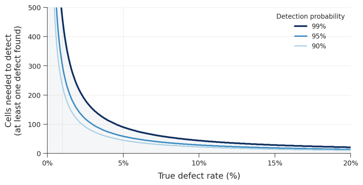
The math is straightforward: the probability of finding at least one defective cell in n inspections is 1 − (1−p)ⁿ. Setting this equal to a target detection probability P and solving for n gives n = ln(1−P) / ln(1−p). This is the same formula as the binomial (∞) curve in Figure 1.
The steep curves on the left of the plot illustrate the challenge of sampling at low defect rates. To have a 95% probability of detecting a 1% defect rate, approximately 300 cells must be inspected. At a 5% defect rate, only 59 cells are needed. This is how the choice of inspection threshold (defined by the pass/fail criteria) determines the required sample size. The same math sets a practical floor on what sampling can demonstrate: bounding a defect rate of 100 ppm (0.01%) at 95% confidence requires about 30,000 cells, and 1 ppm requires about 3 million. For defect modes this rare, demonstrating such a low upper confidence bound by sampling alone may require impractically large sample sizes; it must be paired with process controls at the supplier, inspection approaching 100% coverage, or both.
Sample size is only half the story; the other half is producer’s risk, the chance of rejecting a good lot (see “Acceptance Sampling Standards” above). A c = 0 plan rejects every lot in which a defect is found, including lots whose true defect rate is well below the target. For example, the 299-cell plan that rejects a 1% defect rate with 95% confidence also rejects a lot with a true 0.5% defect rate about 78% of the time and a 0.1% lot about 26% of the time. Plans that allow a few defects (c > 0) reject fewer good lots, but they need more cells for the same consumer protection: bounding a 5% defect rate at 95% confidence takes 59 cells with c = 0, 93 cells with c = 1, and 124 cells with c = 2. For safety-critical defects, we consider this tradeoff worthwhile: a wrongly rejected lot costs time and money, but a wrongly accepted lot can cost far more in the field.
A c = 0 plan can terminate early in only one direction. Because the first defect rejects the lot, inspection can stop as soon as a defect is found, which saves testing time on bad lots without changing the statistics. This practice is known as curtailed inspection. Accepting a lot, however, always requires inspecting all n cells with zero defects: stopping at 150 of 299 cells, for example, bounds the defect rate at about 2% rather than 1% for a large lot. Likewise, a lot should not be “salvaged” by scanning additional cells after a defect is found, since repeated attempts inflate the chance of accepting a bad lot. For early decisions in both directions, use a plan designed for them, such as the double and multiple sampling plans in ANSI/ASQ Z1.4 or the adaptive methods discussed below.
Advanced Methods for Acceptance Sampling
The methodology presented here is a simple form of acceptance sampling. The math assumes binary pass/fail inspection of independent cells, and the statistical framework is well-established, codified in widely-cited standards documents, and has been used in manufacturing quality control for decades. This method is known as attribute sampling. Overall, we recommend our simple approach as a starting point for a battery IQC program.
However, sampling approaches can be far more sophisticated than what we’ve shown here. Attribute sampling as defined in the ISO 2859-1 and ANSI/ASQ Z1.4 standards incorporate additional features beyond what we presented here, including AQL indexing, inspection levels, switching rules, and single/double/multiple sampling plans. Many resources are available online (e.g., here for AQL-indexed plans). Furthermore, because attribute sampling assumes independent samples evaluated via a pass/fail decision, it is not as information-efficient as alternative approaches that extract more information from each inspected cell, update the required sample size dynamically as data accumulates, or both.
A common extension is variables sampling, codified in ISO 3951 and ANSI/ASQ Z1.9. When the inspection yields a continuous measurement rather than a binary pass/fail — such as OCV, internal resistance, capacity, or a scalar geometric dimension from CT — this additional information can be exploited statistically. Variables sampling plans can require fewer cells than binary plans for the same statistical confidence level, because a continuous measurement carries more information than a single bit (e.g., pass/fail). The efficiency gain can be substantial, but only if the measurements follow the distribution that the plan assumes (typically normal). This assumption deserves scrutiny for defects driven by the tail of the distribution. Variables plans also assume measurement error is small relative to the cell-to-cell variation, which is not always the case for CT-derived geometric dimensions.
A more advanced extension is what we call “distributional sampling”, which applies when the inspection yields not a single number per cell but a full distribution of measurements. CT scanning provides exactly this: anode overhang, for example, can be measured at thousands of angular positions and windings for each cell. The distribution of those measurements is far more informative than a single scalar value (although measurements within a cell are correlated, so the effective sample size is still primarily limited by the variation between cells). Methods such as hierarchical Bayesian models can use the initial few scans to learn the between-cell and within-cell variance structure, then update the required sample size adaptively as data accumulates. In principle, this approach can substantially reduce n relative to variables sampling approaches.
Glimpse is actively developing these distributional methods for battery cells to best leverage the rich spatial data that CT scanning provides. However, our work on this so far is not yet validated for production use, and we do not recommend them as the basis for an IQC program at this time. For customers deploying lot acceptance testing today, the standard binary methodology described in this document is a great starting point. As Glimpse’s advanced methods mature, we will publish updated guidance.
How Glimpse Enables High-Throughput Lot Qualification
Glimpse provides high-throughput CT scanning and an automated inspection algorithm suite designed for battery cell inspection at production scale. Unlike conventional CT systems with scan times of hours per cell, Glimpse’s software reduces scan time to minutes per cell with standard CT scanners and seconds per cell with state-of-the-art scanners, making statistically rigorous sampling plans with n = 50 to 500 cells feasible within a standard receiving window.
Glimpse’s algorithm suite automatically extracts the geometric and structural measurements required for lot qualification, including anode overhang violations, core buckling and impingement, can dents, and more, and outputs a pass/fail decision against user-defined specification limits. Glimpse can also develop bespoke computer vision algorithms upon request. Our solution enables the sampling plans described here.
The question of how many cells must be scanned to qualify a lot was a key topic in our presentation at the 2025 NASA Aerospace Battery Workshop. NASA’s 2017 work instruction (EP-WI-036B) specified CT scanning of 14 cells from a 60,000-cell lot. Under the framework in this document, 14 cells provide only a 51% probability of detecting a 5% defect rate, well below NASA’s 90% minimum confidence standard; reaching 90% requires 45 cells, and 95% requires 59. (EP-WI-036B derives sample sizes from a margin-of-error formula for estimating a proportion, which answers a different question than lot acceptance; our presentation at the workshop used the work instruction as-is.) Glimpse’s technology enables the sample sizes shown in Tables 1 and 2 well within practical time and cost constraints.