Get the most out of your scans by learning the fundamentals of CT theory. Read about contrast, voxel size, resolution, and image quality.

CT stands for “computed tomography”. You might know CT by its old name, “computed axial tomography”, or “CAT” scanning. In short, X-ray CT is 3D X-ray imaging. You’ve encountered CT imaging if you’ve ever had a medical CT scan for an injury or illness, or if you’ve had your luggage inspected during an airport security screening.
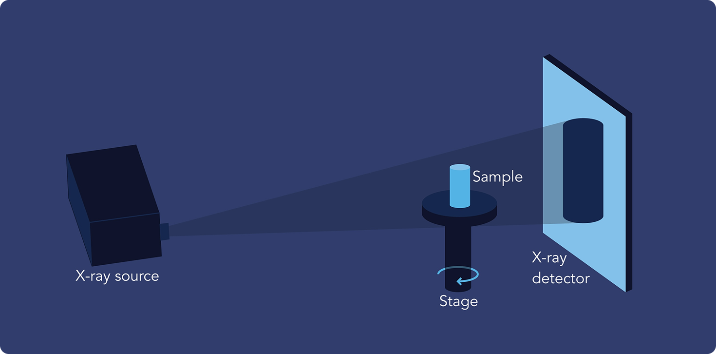
In X-ray imaging, X-rays are first generated by an X-ray source. The X-rays pass through the sample and are detected by an X-ray detector. The sample rotates on a stage during scanning, producing a sequence of hundreds or thousands of 2D X-ray images.

These 2D X-ray images (termed radiographs or projections) are then reconstructed into a 3D volume that approximates the sample. A schematic of the basic geometry of a CT scanner is shown above.
The contrast in CT comes from differences in radiodensity, which is a measure of how strongly X-rays are attenuated by a material. Higher radiodensity means brighter pixels in CT images.
While the various interactions between X-rays and matter can get complicated, for our purposes we can assume that X-rays will interact most strongly when many electrons are present. The number of electrons comes from two key factors:
These contributions to radiodensity are captured by the attenuation coefficient. The mass attenuation coefficient is measured in units of m²/kg or cm²/g.
Note that industrial CT grayscale values are not typically scaled to standard units such as Hounsfield units (HU), which are used in medical CT. To estimate density, the grayscale values of a sample can be compared to the grayscale values of reference materials with known density and composition.
Image quality is a complex topic, especially in CT. Some important attributes of image quality for CT include:
While some quantitative metrics for comparing the quality of two images exist, such as the structural similarity index measure (SSIM) or peak signal-to-noise ratio (PSNR), these metrics do not capture all aspects of image quality. Moreover, the “best” image quality depends on the specific use case; for instance, detecting difficult features such as small metallic particle contaminants may place strict demands on spatial resolution.
Of course, all of these factors must be balanced against the need for fast scan times. You can learn more about the tradeoff between image quality and scan time in our blog post.
A voxel is a “volume element”, analogous to a pixel (“picture element”) in a 2D image. Voxel size is the size of a single 3D pixel in a reconstructed volume. The voxel size can be readily determined from the scan parameters.
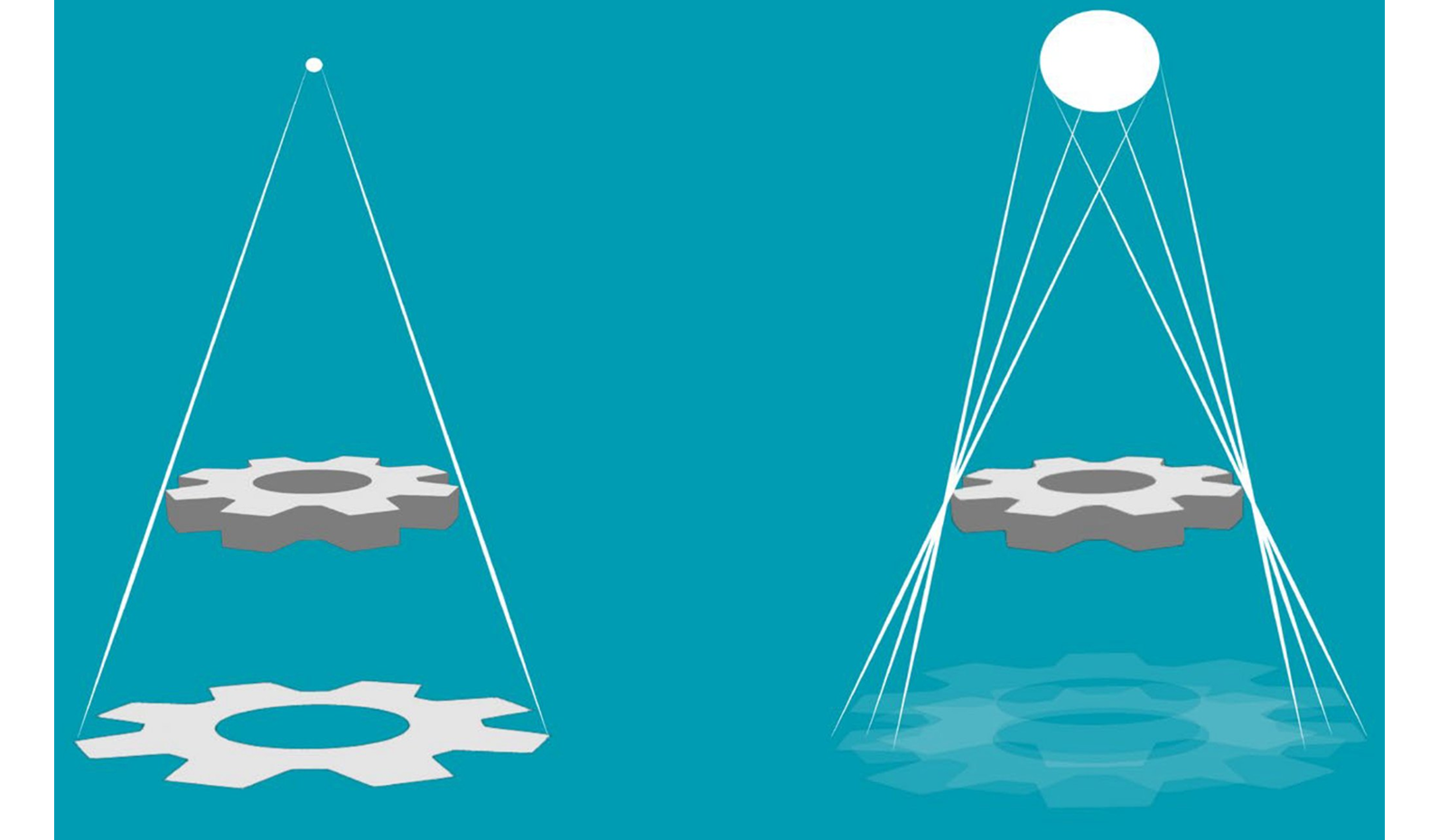
Resolution is a measure of our ability to resolve small details in a scan. Resolution depends on many factors: the focal spot size of the X-ray source, detector pixel pitch, system geometry, motion blur, reconstruction algorithm, and more. In practice, resolution determines what features we can reliably observe — for example, whether a metallic particle contaminant is visible. That’s why resolution, not just voxel size, is the more relevant metric in CT imaging. To accurately quantify resolution, a standard such as a calibrated resolution phantom is needed to provide a consistent, objective benchmark to determine what feature sizes can be reliably resolved in a CT scan.
While the voxel size contributes to resolution, the resolution cannot be determined by the voxel size alone. A feature must have a characteristic length of 3-5x the voxel size to be detected; this requirement increases to 5-20x to quantify feature morphology. For instance, to resolve a feature with a characteristic length of 100 µm, the voxel size should be no larger than 20-33 µm for visualization and 5-20 µm for quantification.
This blog post offers an accessible introduction to this topic.
Short answer: Many factors drive voxel size and resolution, and slower scans generally do not unlock improved voxel size/resolution.
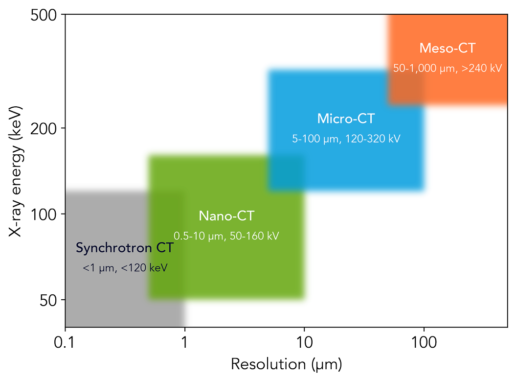
Longer answer: First, keep in mind that CT scanners are designed for specific applications. Specifically, CT scanners are often classified as nano-CT, micro-CT, or meso-CT systems (reference):

Each of these systems is designed to operate within a specific range of voxel sizes and resolutions. The specific design considerations for voxel size and resolution include:

Due to all of these limitations, especially 1–3 above, slower scans generally do not unlock significantly improved voxel size/resolution. Read here to learn more.
While the Glimpse Portal is compatible with nearly all CT scans, Glimpse’s own CT scanners are micro-CT systems. As such, the minimum focal spot size of our X-ray sources limits the minimum practical voxel size of our scans to about 5 µm. However, this voxel size can only be achieved for very small samples.
Two options for scanning with <5 µm voxel sizes include:
In practice, CT reconstruction yields an approximation of the sample, albeit generally a very good one. Deviations between the reconstructed volume and the sample primarily occur due to CT artifacts (learn more here).
Some common CT artifacts include:
Metal streaking artifacts: Metal streaking artifacts occur when X-rays pass through dense metallic components. These artifacts are common and largely unavoidable. Read more here.
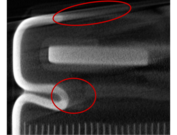
Twinning, windmill, geometric calibration, or center of rotation artifacts: This family of artifacts occurs either when slight miscalibrations of the scanner are not corrected during reconstruction or when the stage/sample moves during scanning. Often, this artifact will manifest as blurriness that varies across the scan. These artifacts can be minimized with proper system calibration, sample fixturing, and reconstruction optimization. Read more here and here.
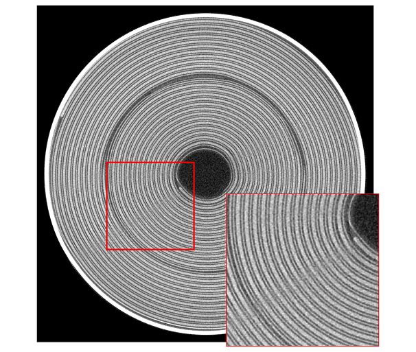
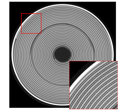
Undersampling or aliasing artifacts: Undersampling or aliasing artifacts occur at the outer edges of the scan when too few projection images are collected. This artifact can be avoided by acquiring more projections, at the expense of a longer scan time. Read more here.
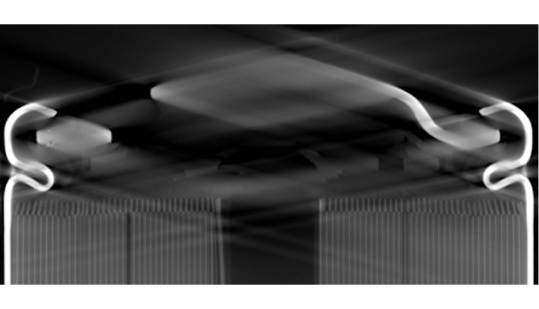
Cone beam artifacts: Cone beam artifacts occur at the top and bottom of a scan when using conventional cone beam geometry and reconstruction algorithm (circular scanning). This artifact can be avoided with helical scanning, among other techniques. Read more here.
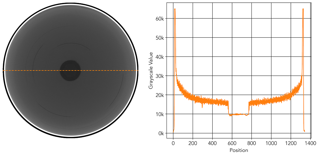
Beam hardening artifacts: Beam hardening artifacts are another common artifact in CT scans. This artifact can be minimized either by filtering the X-ray beam or via software corrections. Read more here.
While Glimpse takes pride in minimizing artifacts in our scans, artifacts can occasionally complicate scan interpretation. Of course, if you have any questions about your scans, don’t be shy in reaching out to us at support@glimp.se.

Learn from our team of battery quality experts what CT can and cannot reveal in your cells, and why.
Our published research on how cells fail and which defects matter.
We are true CT nerds and can talk about the theory behind it for hours. If you have more questions, reach out to our engineering team!
Not sure where to start? Talk to us.